Welcome to the ERTH 304 Rotating Tank webpage for the Fall 2022 semester.
The instructor will try to update this page every few days as the semester progresses.
This semester students and I are experimenting with the rotating tank that was procured a couple years ago with Student Learning Fee funds. The goal is to help students (and instructor!) learn about the dynamics of large-scale atmospheric and oceanic circulations which are profoundly affected by the rotation of the Earth. We follow parts of the book by Marshall and Plumb. We place tracers (colored dye or small floating pieces of paper) in water to reveal fluid motion. A downward pointing video camera is rotating with the tank to enable us to observe the circulations in the rotating reference frame (a.k.a. coordinate system), just like we do when we look at geostationary satellite imagery or weather maps.
The tank represents a rapidly rotating fluid (a fluid may be gas or liquid), similar (believe it or not) to the Earth's atmosphere or oceans. It may not seem like the Earth's atmosphere or oceans are rotating rapidly, but by "rapid" it's important to consider the lifetime of the circulations relative to the rotation rate of the fluid. For Earth's atmosphere or oceans we are dealing with time evolutions of hours to days with rotation rates of once per day. In the tank, we are dealing with circulations that evolve over seconds to minutes while the rotation rate is order several times per minute. [Note: The importance of rotation in the dynamics of a circulation may be quantified by the temporal Rossby number Ro=1/(ΩT) where Ω is the rotation rate and T is the characteristic time scale of the circulation.]
A significant difference between our tank and the real atmosphere is that the Coriolis force does not change with latitude. On Earth, the horizontal Coriolis force is a maximum at the poles and decreases as one moves towards the equator. This is because the surface of the earth is perpendicular to the axis of rotation at the pole and gradually becomes parallel to the axis of rotation at the equator. In the tank, the axis of rotation is perpendicular to horizontal motions everywhere. In this regard, fluid motions in the tank are like those at very high latitudes.
Thus far, we've learned a few practical lessons. First, it's very helpful to fill the tank a day or more in advance to let the water come into thermal equilibrium with the room. Tap water is normally colder than room air temperature and the temperature difference may induce density driven effects that interfere with the experiments. It's also important to allow the fluid to settle into "solid body rotation" and not disturb it with bumps or motions that induce undesirable velocities that interfere with the circulations that we are trying to induce.
9/27/2022: By experimenting, we learned how to generate super-rotation (meaning the fluid circulates around the pole faster than the tank itself and in the same direction) by carefully adding crushed ice to a stainless steel bucket at the pole while the tank was on it's slowest rotation rate. This created a thermally direct circulation cell in the radial dimension by chilling the water near the pole, increasing its density and causing it to sink. In the Earth's atmosphere an energy surplus exists near the equator and a deficit exists near the poles. In our rotating tank, we simply have a deficit near the pole that induces the circulation. This super-rotating flow is geostrophic and sheared in the vertical (i.e., a "thermal wind" is present.)
Doing this at the slowest rotation rate results in a stable baroclinic fluid. Without the ice bucket at the pole, one has a barotropic fluid because the density of the water is only a function of depth and pressure (the isobars and isopycnals in the vertical plane are parallel). By chilling the water near the pole, we induce tilted isopycnic surfaces that intersect nearly-horizontal isobaric surfaces and create what is known as a baroclinic fluid. At the slowest rotation rate of the apparatus, we see concentric rings of dye (shown below). By speeding up the rotation rate we expect to observe baroclinic instabilties like the ones observed in the large-scale mid- and high latitude atmospheric circulations.
Moreover, we see the water at the top moving the fastest (in super-rotation). Side views reveal injected columns of dye tilting over showing the vertical shear of the geostrophic wind (a.k.a., the thermal wind). These are tilted Taylor-Proudman columns.
By carefully increasing the rotation rate, we expect to create baroclinic instabilities soon. We also plan to investigate Ekman layers and fronts, and demonstrate how Taylor-Proudman tends to cause flow move along contours of constant depth.
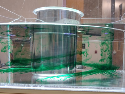
10/18/2022: In the following animation, we lift a open-ended cylinder to release a slightly denser fluid (1 tablespoon of salt dissolved) with green dye and watch how rapidly the negatively buoyant fluid spreads out in the bottom of the tank. This is done with a non-rotating system. In the future we plan to repeat the experiment but with rotation on to see the constraining effect of the rotation.
10/26/2022: Now, compare that to what happens with rotation:
The rotation "stiffens the fluid" causing it to resist shearing and deformation. The high density fluid (salty water with green dye) does not slump to cover the entire bottom of the tank. Rather is it constrained to maintain a bell shape.
The salty "green blob" is a higher density fluid, much like a cold polar atmosphere at high latitudes. Rather than continuing to spread out and cover the bottom of the tank uniformly and reach a "normal" statically stable equilibrium with dense covering the bottom and light on the top, rotation constrains the blobs ability to fully slump as intuition would expect.
Yet, the blob is no longer anchored to the "pole" (the axis of rotation) by the metal cylinder. The imperfect release of the blob from the cylinder and perhaps very small, inadvertent, large scale circulations in the tank allows it to slowly migrate to a position that it is no longer centered on the axis of rotation. Yet, it stays together on a horizontal scale roughly the same as the diameter of the can as shown below almost 10 minutes after release.
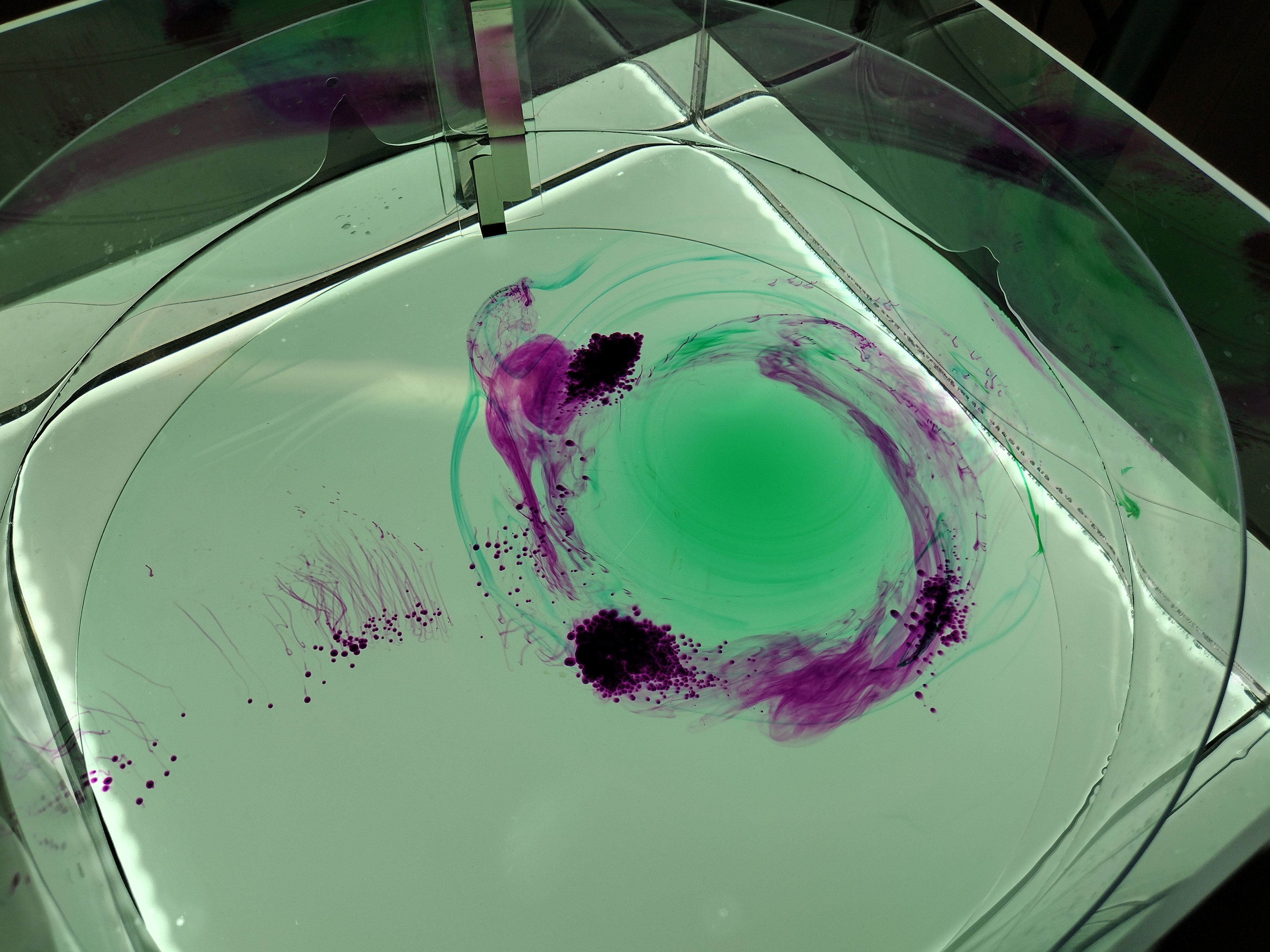
Note how the purple dye circulates around the green blob but generally resists mixing with it. Moral of the story: rotating fluids resist 3D mixing in ways that we intuitively expect.
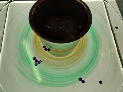
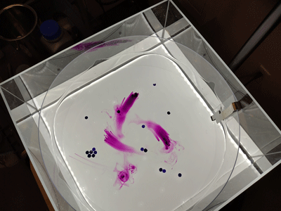
10/27/2022: We pulled off the Ekman experiment today. Brought the tank into solid body rotation then turned down the rotation rate just slightly to induce super-rotation. We dropped gains of potassium permanganate that fall to the bottom and slowly dissolve leaving purple streaks that reveal converging fluid. The explanation for this is we have (a) induced geostrophic flow by slowing down the tank and letting inertia put the fluid into super-rotation. This implies a pressure deficit (relative to equilibrium) is at the center of the tank and a pressure surplus exists around the rim. The outward pointing Coriolis force balances the inward PGF except (b) fluid parcels near the bottom (in the boundary layer) are influenced by the friction of the bottom and result in a trio of forces: PGF, Coriolis, and friction, with the resultant flow cutting across isobars toward low pressure.
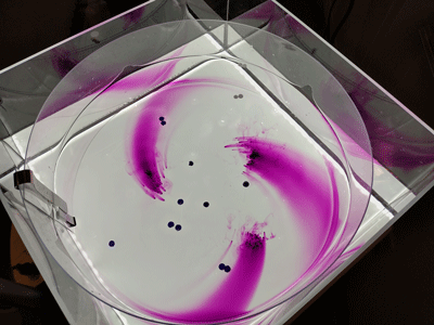
11/01/2022: Today we repeated the Ekman experiment, but this time increased the rotation rate (rather than decreasing it) to induce divergent Ekman flow in the bottom boundary layer. (We also ordered a GoPro Hero10 camera!)
The question comes up: why do we generate low pressure at the center of the rotating tank? The answer is that rotation causes a parabolic surface of water with slightly deeper water around the edges and slightly shallower water at the center. This happens even when the flow is in solid-body rotation. At any constant height above the flat bottom, the pressure is proportional to the height of the water above that level.
When we change the rotation rate, it takes time to bring the fluid to a new equilibrium (a new solution to solid body rotation at that rate). The key is that speeding up the rotation rate results in a pressure surplus at the center and slowing down results in a pressure deficit at the center, relative to that of the new equilibrium. In this way, by generating departures from equilibrium, we can simulate PGFs that point inward and outward, respectively.
The next question is: How can we say that the flow during these adjustment periods is geostrophic?
Dr. Mayor's page