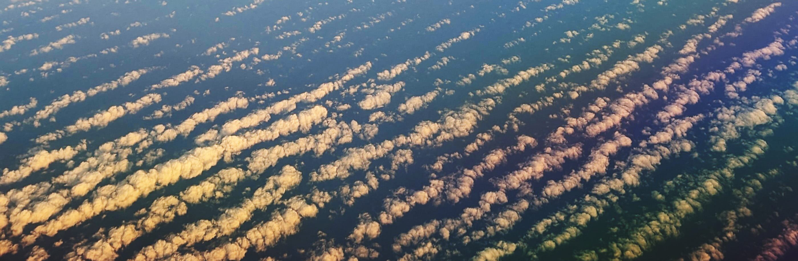
Cloud streets over the western Pacific ocean as viewed from an airliner on 15 July 2026. Photo by S. D. Mayor.
The instructor will try to update this page every few days during the semester. Here is a link to a post on LinkedIn that I made about this class.
Cloud streets over the western Pacific ocean as viewed from an airliner on 15 July 2026. Photo by S. D. Mayor.
Fall 2026 Lectures: MWF, 9:00 - 9:50 AM.
Mon., 24 Aug., Overview of the M2HATS field campaign, observing systems, semester research goals, and AMS 2027 poster project.
Weds., 26 Aug., M2HATS recap; important acronyms and organizations including AMS,
NCAR, and
NSF and federal funding.
Fri., 28 Aug., Computational lab: Begin steps to use ChatGPT and MATLAB to access M2HATS in-situ data; file paths, filenames, extensions, and
Markdown handoff files.
Mon., 31 Aug., Introduced Unidata and netCDF, reviewed the M2HATS ISFS data products and observing-system acronyms, and began the atmospheric boundary layer definition from Stull.
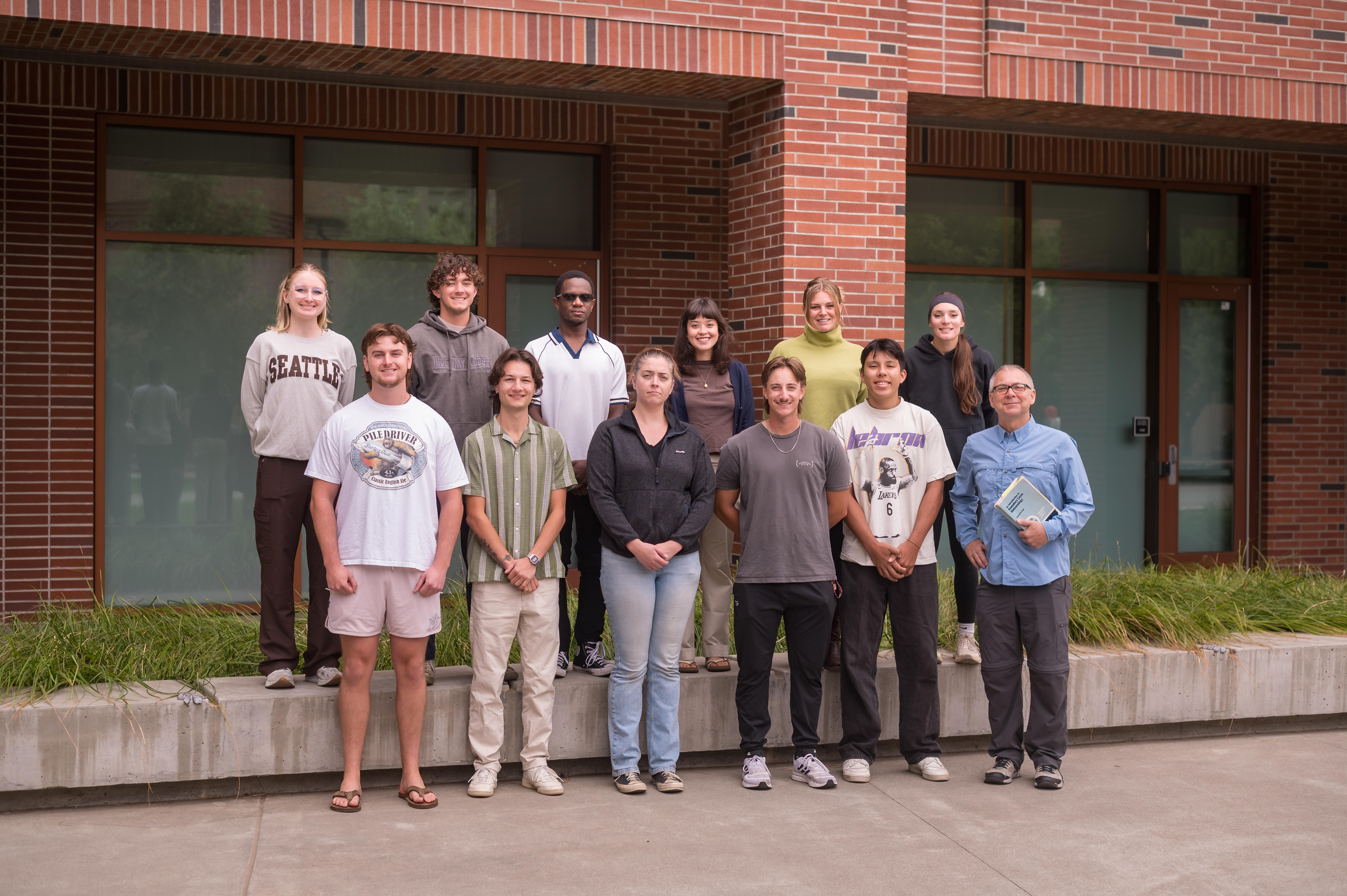
Weds., 2 Sept., Class portrait taken by Jason Halley. Then lecture on structure of the convective boundary layer (CBL).
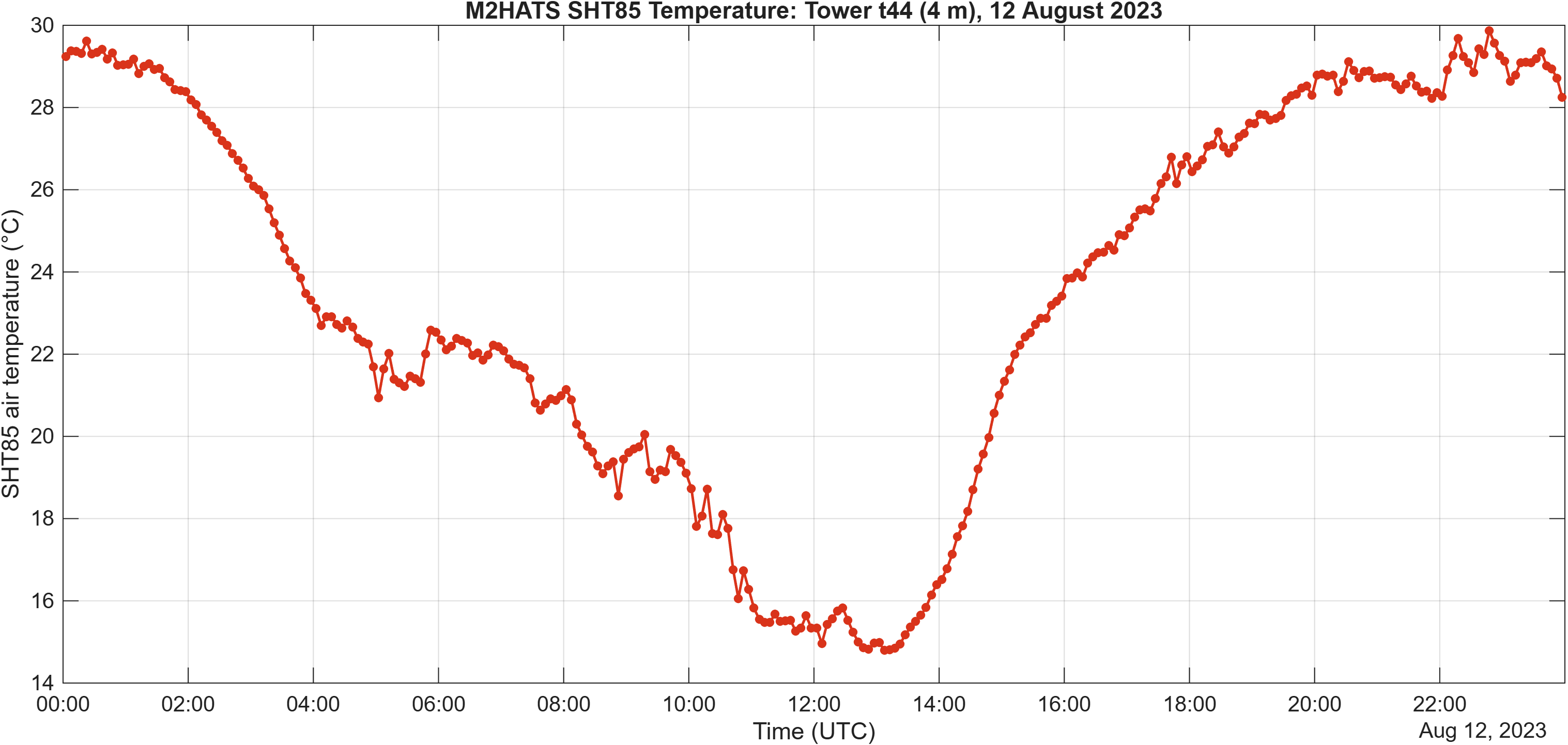
Fri., 4 Sept., Computational lab: Use ChatGPT and MATLAB to make time-series
plot of the diurnal temperature cycle.
Mon., 7 Sept., Labor Day. No classes.
Weds., 9 Sept., Continued discussion of the CBL with emphasis on entrainment and the entrainment zone, convection cells, plumes, and thermals.
Fri., 11 Sept., Computational lab: Use ChatGPT and MATLAB to compare 1-s and 5-min temperature and horizontal wind-speed data and examine the high-rate u, v, and w wind components.
Mon., 14 Sept., Reynolds decomposition, mean and perturbation quantities, variance and standard deviation, and the relationship between velocity variance and kinetic energy.
Weds., 16 Sept., Decomposed kinetic energy into mean kinetic energy (MKE) and turbulent kinetic energy (TKE); calculated variance and standard deviation from perturbations and introduced covariance.
Fri., 18 Sept., Computational lab: Creation of a plot of TKE over the diurnal cycle. Discussion of moments
Mon., 21 Sept., Reviewed variance and covariance, related covariance to turbulent transport, and introduced kinematic versus physical fluxes of sensible heat, water vapor, trace gases, and momentum.
Weds., 23 Sept., Converted kinematic moisture and momentum fluxes to physical fluxes, introduced turbulent stress, and related vertical momentum transport to surface drag.
Fri., 25 Sept., Computational lab: Part 1: plotting sensible and latent fluxes before and after rain. Part 2: Hunting for dust devils in REAL data.
Mon., 28 Sept., Quiz #1. Lecture on fluxes of sensible heat, water vapor mass, latent energy, and momentum.
Weds., 30 Sept., Introduction to u-star (friction velocity) and the log-wind profile.
Fri., 2 Oct., Computational lab: A tour of the Raman-shifted Eye-safe Aerosol Lidar (REAL). Students visited and went inside the REAL.
Mon., 5 Oct., Logarithmic wind profile, friction velocity, mechanical versus convective turbulence, and beginning the derivation of potential temperature.
Weds., 7 Oct., Completion of the potential-temperature derivation, ideal gas law, dry-air gas constant, virtual temperature, and virtual potential temperature.
Fri., 9 Oct., Computational lab: Discussion about REAL imagery from M2HATS and identification of aerosol features in REAL images
Mon., 12 Oct., Introduction to static stability; derivation of hydrostatic balance and beginning of the barometric law.
Weds., 14 Oct., Complete derivation of barometric law and dry adiabatic lapse rate, and evaluate static stability of isothermal atmosphere from density differences.
Fri., 16 Oct., Computational lab: Discussion of 2027 annual AMS meeting and boundary layer and turbulence symposium poster presentation.
Mon., 19 Oct., Neutral and unstable static stability; using environmental and dry adiabatic lapse rates to evaluate stability without calculating displaced parcel densities.
Weds., 21 Oct., Making the leap from temperature lapse rates to potential temperature slopes to evaluate static stability.
Fri., 23 Oct., Computational lab: Discussed examples of theta profiles in Stull's book.
Mon., 26 Oct.,
Weds., 28 Oct.,
Fri., 30 Oct.,
Mon., 2 Nov.,
Weds., 4 Nov.,
Fri., 6 Nov.,
Mon., 9 Nov.,
Weds., 11 Nov., Veterans Day. No classes.
Fri., 13 Nov.,
Mon., 16 Nov.,
Weds., 18 Nov.,
Fri., 20 Nov.,
Mon., 23 Nov., Fall Break. No classes.
Weds., 25 Nov., Fall Break. No classes.
Fri., 27 Nov., Fall Break. No classes.
Mon., 30 Nov.,
Weds., 2 Dec.,
Fri., 4 Dec.,
Mon., 7 Dec.,
Weds., 9 Dec.,
Fri., 11 Dec.,
Mon., 14 Dec., Final comprehensive exam, 10:00 - 11:50 AM.